Compound V2: Interest Rate Models

This article is part of the Compound V2 series. See the series index for a full list of articles.

A previous article showed that the borrow index updates each block as:

newBorrowIndex = oldBorrowIndex * (1 + borrowRate)

That article never explained where the borrow rate comes from. It is determined by the interest rate model, and Compound V2 has several implementations. Each offers a different tradeoff between capital efficiency and liquidity protection. Governance can assign different models to different markets. This article starts with the shared building blocks (utilization rate, supply rate) then walks through each borrow rate model: WhitePaper, JumpRate, and JumpRateV2.

This article ignores fixed-point math details to focus on the underlying formulas.

Utilization Rate

The first concept to understand is utilization, the ratio of underlying assets currently being borrowed.

utilization = borrows / (cash + borrows - reserves)

All values are in underlying asset units.

• borrows: the total amount of underlying assets currently being borrowed
• cash: the cToken contract’s underlying token balance
• reserves: the portion of the cToken contract’s underlying balance that belongs to the protocol, not the market

The denominator (cash + borrows - reserves) is the total assets in the market. cash + borrows is everything the market controls, what’s sitting in the contract + what’s been lent out. Reserves are subtracted because they belong to the protocol, not lenders. Utilization is then the portion of market assets currently being borrowed.

For example, suppose the contract holds 800 USDC in cash, 200 USDC is borrowed, and there are no reserves.

totalMarket = 800 + 200 = 1000 USDC
utilization = 200 / 1000 = 20%

Here is the code implementation:

function utilizationRate(
    uint cash,
    uint borrows,
    uint reserves
) public pure returns (uint) {
    // Utilization rate is 0 when there are no borrows
    if (borrows == 0) {
        return 0;
    }

    return borrows * BASE / (cash + borrows - reserves);
}

The BASE constant (1e18) is for fixed-point math. The result is a value scaled to 18 decimals, where 1e18 represents 100% utilization.

The Interface

All interest rate models inherit from InterestRateModel.sol, an abstract contract with two functions, getBorrowRate and getSupplyRate. Some models implement getBorrowRate differently, but getSupplyRate stays the same across all of them.

WhitePaper Model (Linear Borrow Rate)

The WhitePaper model implements the interest rate formula from the original Compound white paper. The borrow rate scales linearly with utilization. More borrowing means higher rates, as you’d expect from supply and demand.

function getBorrowRate(
    uint cash,
    uint borrows,
    uint reserves
) override public view returns (uint) {
    uint ur = utilizationRate(cash, borrows, reserves);
    return (ur * multiplierPerBlock / BASE) + baseRatePerBlock;
}

This is a simple linear equation:

y = mx + b

• b = baseRatePerBlock: the minimum borrow rate, even when nobody is borrowing
• m = multiplierPerBlock: how steeply the rate increases as utilization rises
• x = utilization rate
• y = borrow rate

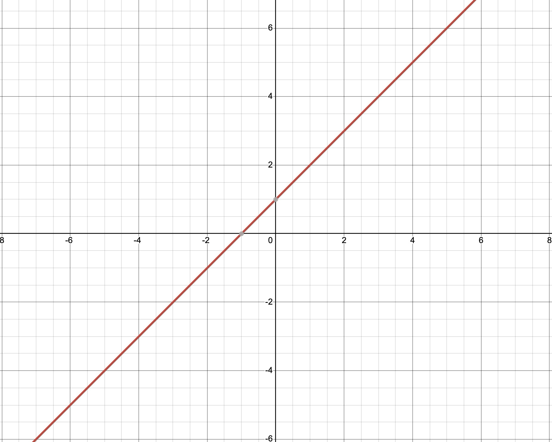
Borrow rate (y) increases linearly with utilization (x).

Supply Rate

The borrow rate is how much interest borrowers pay on their loans. The supply rate is how much yield lenders earn on their supplied assets. The supply rate depends on three factors:

• Borrow rate: the interest rate borrowers are paying
• Reserve factor: the protocol’s cut of the interest
• Utilization: how many assets are actually being borrowed vs. sitting idle

function getSupplyRate(
    uint cash,
    uint borrows,
    uint reserves,
    uint reserveFactorMantissa
) override public view returns (uint) {
    uint oneMinusReserveFactor = BASE - reserveFactorMantissa;
    uint borrowRate = getBorrowRate(cash, borrows, reserves);
    uint rateToPool = borrowRate * oneMinusReserveFactor / BASE;
    return utilizationRate(cash, borrows, reserves) * rateToPool / BASE;
}

The formula is:

supplyRate = utilization * borrowRate * (1 - reserveFactor)

Take the borrow rate, multiply by the portion that belongs to lenders (1 - reserveFactor), then multiply by utilization since not all deposited assets are earning interest, only borrowed ones are.

Say 100 ETH is deposited and 10 ETH is borrowed at a 10% borrow rate, with a 20% reserve factor.

interest generated   = 10 ETH * 10%        = 1 ETH per year
protocol reserves    = 1 ETH * 20%         = 0.2 ETH
remaining for lenders = 1 ETH - 0.2 ETH    = 0.8 ETH
supply rate          = 0.8 ETH / 100 ETH   = 0.8%

Verifying with the formula:

supplyRate = 10% * 10% * (1 - 20%) = 0.8%

JumpRate Model (The Kink)

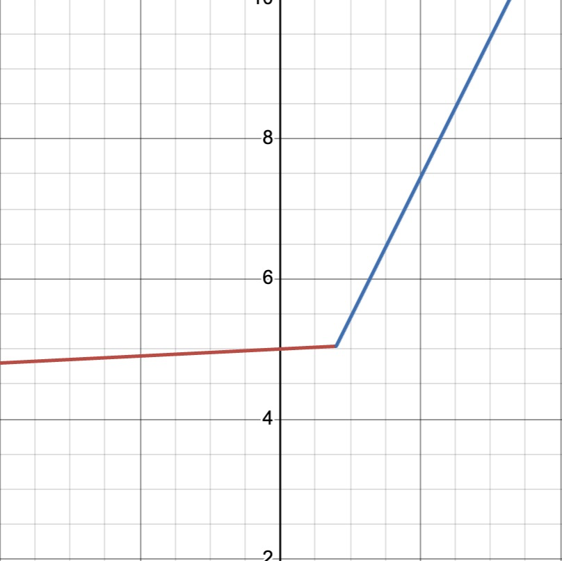
A single linear model treats 20% utilization and 95% utilization with the same urgency. At very high utilization, the protocol needs to aggressively discourage borrowing and incentivize new supply, otherwise the market runs out of liquidity for withdrawals. The JumpRate model solves this with a kink, a utilization threshold where the interest rate curve gets steeper.

Below the kink, the formula is the same as the WhitePaper model. Above it, rates rise much faster to:

• Discourage additional borrowing
• Encourage lenders to supply more assets
• Prevent 100% utilization, which would leave no liquidity for withdrawals

Both segments are still linear, just with different slopes.

function getBorrowRate(
    uint cash,
    uint borrows,
    uint reserves
) override public view returns (uint) {
    uint util = utilizationRate(cash, borrows, reserves);

    if (util <= kink) {
        return (util * multiplierPerBlock / BASE) + baseRatePerBlock;
    } else {
        uint normalRate = (kink * multiplierPerBlock / BASE) + baseRatePerBlock;
        uint excessUtil = util - kink;
        return (excessUtil * jumpMultiplierPerBlock / BASE) + normalRate;
    }
}

Below the kink, this is the familiar y = mx + b:

rate = baseRate + multiplier * utilization

Above the kink, the goal is to create a second line with a steeper slope that connects with the original line. Simply changing m would disconnect the two segments. They need to meet at the kink point.

The trick is to treat the kink as the new origin for the second line. The rate at the kink is computed using the first formula:

normalRate = baseRate + multiplier * kink

normalRate becomes the y-intercept b of the second line. Then (utilization - kink) is used as the x value, which is zero at the kink and grows from there. At the kink, m is multiplied by zero and produces zero. The only thing left is + normalRate, which is the same value the first line produces at that point. Both lines end up with a different slope but the same y value at the kink. This guarantees the two segments connect.

rate = jumpMultiplier * (utilization - kink) + normalRate

Say baseRate = 1, multiplier = 2, jumpMultiplier = 5, and kink = 4. At the kink, both formulas should give the same rate.

line 1: rate = 1 + 2 * 4           = 9
line 2: rate = 5 * (4 - 4) + 9     = 5 * 0 + 9 = 9

Both lines produce 9 at the kink. Above it, jumpMultiplier kicks in. At utilization = 5:

line 2: rate = 5 * (5 - 4) + 9     = 5 * 1 + 9 = 14

If this doesn’t click, try drawing it on graph paper. Draw the first line, pick a steeper slope, and figure out how to make it connect at the kink. Working through it yourself makes it stick.

JumpRateV2 (Updatable Parameters)

JumpRateV2 inherits all its logic from BaseJumpRateModelV2. The rate calculations are identical to the JumpRate model. The only difference is that an admin can update the parameters without deploying a new contract.

In the original JumpRate model, governance had to deploy a new contract and point the market to it. JumpRateV2 adds updateJumpRateModelInternal to update parameters in place:

function updateJumpRateModelInternal(
    uint baseRatePerYear,
    uint multiplierPerYear,
    uint jumpMultiplierPerYear,
    uint kink_
) internal {
    baseRatePerBlock = baseRatePerYear / blocksPerYear;
    multiplierPerBlock = (multiplierPerYear * BASE) / (blocksPerYear * kink_);
    jumpMultiplierPerBlock = jumpMultiplierPerYear / blocksPerYear;
    kink = kink_;

    emit NewInterestParams(baseRatePerBlock, multiplierPerBlock, jumpMultiplierPerBlock, kink);
}

There is a subtle difference in how V2 stores multiplierPerBlock compared to V1.

V1 (JumpRateModel.sol):

multiplierPerBlock = multiplierPerYear / blocksPerYear

V2 (BaseJumpRateModelV2.sol):

multiplierPerBlock = (multiplierPerYear * BASE) / (blocksPerYear * kink_)

V2 divides by the kink when storing the multiplier. This changes what number you pass in as multiplierPerYear, but both versions produce the same borrow rate curve.

Suppose you want the borrow rate at the kink to be 10% (annualized), with a kink at 50% utilization and a base rate of 0%.

The rate at the kink is:

rateAtKink = baseRate + multiplier * kink

V1: You do the math yourself.

10% = 0 + multiplierPerYear * 50%
multiplierPerYear = 20%

You pass 20% into the constructor.

V2: The contract does the math for you. You pass multiplierPerYear = 10%. The contract divides by the kink internally:

10% / 50% = 20%

It stores that.

Both end up storing the same effective multiplierPerBlock. Both produce a 10% rate at the kink. The difference is just the interface. V1 wants the raw slope (20%), V2 wants the rate at the kink (10%).

Conclusion

All of Compound’s interest rate models share the same utilization rate and supply rate logic. They only differ in how the borrow rate scales with utilization. The WhitePaper model uses a single linear curve, the JumpRate model adds a kink to protect liquidity at high utilization, and JumpRateV2 makes the parameters updatable without redeploying the contract.